3D Model of Tutte's 8-cage

by François Labelle

Final Project presented to Carlo Séquin

for CS294-3 Rapid Prototyping, Fall 2000

1. Introduction

For my final project, I wanted to build a pleasing 3D model representing a fairly large combinatorial graph of some theoretical importance.

I quickly found out that the graph should have low degree, preferably 3 or 4, to obtain a nice uncluttered 3D model. Also, I thought that it would be nice if the graph had some properties that could be verified by inspection. This suggested that I choose a graph from the family of (3,n)-cages, which are graphs of uniform degree 3 (also called "cubic") such that the smallest cycle in the graph has n vertices. In other words, starting from any vertex and making any sequence of n-1 moves (but no U-turn), you are guaranteed to visit n distinct vertices.

Why Tutte's 8-cage?

Tutte's 8-cage, also known as the Tutte-Coxeter graph, has 30 vertices and 45 edges. It is the unique smallest (3,8)-cage. For comparison, the Petersen graph has 10 vertices and is the unique smallest (3,5)-cage. I tried larger cages but it was too difficult to get nice 3D embeddings of them. Cages starting from parameters (3,9) are not always unique, which makes the (3,8) case somewhat special. More information about cubic cages is available at http://www.cs.uwa.edu.au/~gordon/cages/.

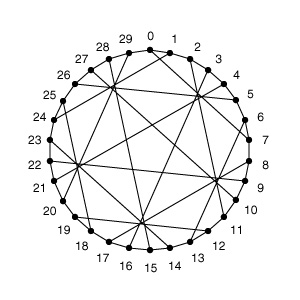
Tutte's 8-cage is usually drawn as shown below (image from http://www.pbase.com/image/15584). The drawing is already nice and symmetrical, but a 3D model can ideally have edges of similar length and no crossings.

Figure 1. Tutte's 8-cage drawn in 2D.

2. From combinatorics to geometry

Recall that a graph is just an abstract set of vertices and edges, with no coordinates attached to them. A graph embedding is a mapping from the set V of vertices to R^d for some dimension d = 1,2,3,4,.... Edges follow.

Example:
n=8, m=8
V = {1,2,3,4,5,6,7,8}
E = {(1,2), (2,3), (3,4), (4,1), (1,5), (2,6), (3,7), (4,8)}

Figure 2. Two possible 2D embeddings of the example graph.

As seen in Figure 2, no notion of quality has been introduced yet. Since the embedding on the left is clearly more desirable, we introduce some common sense rules. In a good embedding...

graph distances should play a role,
graph symmetries should be visible,
edges and vertices should not overlap.

3. Electrical distance embedding

The usual definition of graph distance between two vertices is the number of edges on the shortest path between the two vertices. This will be contrasted with an alternate definition based on electrical circuits.

graph		electrical circuit
graph distance d(x,y)		effective electrical resistance r(x,y)

Figure 3. Different concepts of graph distance.

The effective electrical resistance satisfies 0 <= r(x,y) <= d(x,y) and turns out to be more useful for my purpose because there exists a unique embedding f : V -> R^n-1 such that

|| f(x) - f(y) || = {r(x,y)}^1/2 for all x,y in V.

But it is not always possible to find f such that

|| f(x) - f(y) || = {d(x,y)}^a for all x,y in V

even for a = 0.0001.

Computing explicit coordinates

Effective electrical resistance can be computed from Ohm's law and the principle that the sum of the currents leaving each node is zero. This amounts to a matrix inversion, which in the case of the example graph gives the following array of distances between pairs of vertices:

   1    2    3    4    5    6    7    8
1  0.00 0.75 1.00 0.75 1.00 1.75 2.00 1.75 
2  0.75 0.00 0.75 1.00 1.75 1.00 1.75 2.00 
3  1.00 0.75 0.00 0.75 2.00 1.75 1.00 1.75 
4  0.75 1.00 0.75 0.00 1.75 2.00 1.75 1.00 
5  1.00 1.75 2.00 1.75 0.00 2.75 3.00 2.75 
6  1.75 1.00 1.75 2.00 2.75 0.00 2.75 3.00 
7  2.00 1.75 1.00 1.75 3.00 2.75 0.00 2.75 
8  1.75 2.00 1.75 1.00 2.75 3.00 2.75 0.00

Table 1. Matrix of effective electrical resistances r(x,y) for the example graph.

Since all the distances are known, one can compute the actual coordinates in a greedy fashion:

assign coordinates (0,0,0,...,0) to vertex 1,
assign coordinates (a,0,0,...,0) to vertex 2, where a = {r(1,2)}^1/2,
assign coordinates (b,c,0,...,0) to vertex 3, where b and c are such that the distances {r(1,3)}^1/2 and {r(2,3)}^1/2 are satified,
etc.

This is equivalent to computing the Cholesky factorization of a corresponding "matrix of inner-products" which can be obtained from the r(x,y) values.

This method is guaranteed to produce coordinates that encapsulate every symmetry of the graph. The only problem is that the embedding lies in n-1 dimensions (where n is the number of vertices). In the case of Tutte's 8-cage, the embedding lies in 29 dimensions.

4. Reduction from 29 dimensions down to 9

The standard technique to reduce the dimensionality of a point-set is Principal Component Analysis, which produces a set of orthogonal axes (called principal components) sorted by their ability to capture the multidimensional data. Explaining the details of Principal Component Analysis would be a final project on its own, and indeed was my final project in a previous course: http://www.cs.mcgill.ca/~sqrt/dimr/dimreduction.html.

Analysis of the example graph:

Eigenvalues and eigenspace dimensions:
 1:  1.707107 (2)  mfs=0.500000
 2:  1.309017 (1)  mfs=0.000000   OVERLAP: 4*[2]
 3:  0.500000 (1)  mfs=0.000000   OVERLAP: 2*[4]
 4:  0.292893 (2)  mfs=0.000000
 5:  0.190983 (1)  mfs=0.000000   OVERLAP: 4*[2]

This is my program crude output. Basically, the first row is the most important, which says that the best fit for the graph is a two-dimensional (2) embedding of quality 1.707107 (this value can be viewed as some constant minus the error made by the dimensionality reduction). The value mfs=0.500000 is the "minimum feature size", which tells me that no vertices/edges overlap in this projection. The last column gives additional information about vertex overlaps (how many groups there are, and how many superposed vertices there are in each group).

The next few rows can sometimes be useful too. The last rows are in some sense the "worst" fit for the graph, in which the edges are likely to run from one end to another. Since the last rows also convey symmetries, they can sometimes give artistic results too.

eigenspace 1

eigenspace 4

Figure 4. Two embeddings of the example graph, produced by the program.

Analysis of Tutte's 8-cage:

Eigenvalues and eigenspace dimensions:
 1:  1.000000 (9)  mfs=0.447214
 2:  0.333333 (10) mfs=0.288675
 3:  0.200000 (9)  mfs=0.105409
 4:  0.166667 (1)  mfs=0.000000   OVERLAP: 2*[15]

As seen from the analysis, Tutte's 8-cage has a beautiful embedding in 9 dimensions. This is a huge step down from 29 dimensions, but still is not enough for my purpose.

Simplification of the overall procedure

It turns out that the 3 steps I have described simplify nicely:

solving the equations of current flow in the electrical circuit,
embedding the graph in R^n-1 with a Cholesky factorization,
doing a Principal Component Analysis of the point-set.

There's no need for a Cholesky factorization if it is to be followed by a PCA, and there's no need for a matrix inversion in step one for the same reason. All one has to do is to construct the Laplacian matrix of the graph (which is the negative of the adjacency matrix, plus the degree of each vertex on the diagonal) and do an eigenvalue/eigenvector decomposition of it, which is how I have implemented it.

       /  3 -1  0 -1 -1  0  0  0 \
       | -1  3 -1  0  0 -1  0  0 |
       |  0 -1  3 -1  0  0 -1  0 |
   L = | -1  0 -1  3  0  0  0 -1 |
       | -1  0  0  0  1  0  0  0 |
       |  0 -1  0  0  0  1  0  0 |
       |  0  0 -1  0  0  0  1  0 |
       \  0  0  0 -1  0  0  0  1 /

Table 2. The Laplacian matrix of the example graph.

5. Reduction from 9 dimensions down to 3

Nine dimensions is as low as Principal Component Analysis would allow me to go. To reduce further, one needs to break some of the symmetries arbitrarily (which PCA won't do). When we embed a 4D-hypercube in 3D, many designs are possible and each one will break some symmetry of the hypercube, but the process is still manageable. A reduction from 9D to 3D is the same principle, but as I have found is much much harder. I have no general procedure for doing this, and so the rest of the process is pretty ad-hoc.

Trying random projections

If there is one very good projection to 3D, then by trying many random projections we can hope that we will hit some projection so close to the optimal that it will itself be a good projection. The optimal projection can then be found by local improvement. This will work for low dimensions and/or small number of vertices. Indeed, this is how I found a good 3D embedding of the Petersen graph (a reduction from 5D to 3D).

However, I wasn't so lucky for Tutte's 8-cage. After doing 470 million random trials, the best projection had a minimum feature size of 0.195 and didn't look symmetric at all. (I achieved a mfs of 0.216 with some human intervention, see later). In short, the search space is too large for a brute force attack.

Enforcing symmetries

After many unfruitful attempts, what turned out to work was to force edges (0,1) and (15,16) to be parallel to the 3D-projection screen (the vertex numbering is as in Figure 1). Doing this reduced the number of degrees of freedom of the projection by about half. A randomized search (as before, but constrained) finally uncovered a projection that I found satisfactory. It is left as a game for the reader to conjecture where the edges (0,1) and (15,16) appear on the final piece.

Although the final shape looks symmetric, it should be noted that most of the symmetries of Tutte's 8-cage are lost! In the graph, every vertex is equivalent, and every edge is equivalent, which I don't think is obvious from the sculpture.

Although every vertex is equivalent, the graph is bipartite and vertices can be naturally split into 2 (equivalent) sets of 15 vertices each. This is what I chose to represent with black and blue vertices.

Below is another view of the chosen 3D embedding, different from the one on the front page.

Figure 5. A view of Tutte's 8-cage showing some symmetries.

6. Choice of the building process

The sculpture can be physically built by any process that can create cage-like structures. I feel it is important to show the duality between vertices and edges as much as possible, so I used contrasting colors and made the vertices twice as large as the edges. For this reason, I think that the Zcorp 3D printer is best suited. The Stratasys FDM machine can also be used to create the part, although the color cues won't be available.

Another possibility would be to generate the edges and vertices separately on the FDM machine with different colors, and to assemble them manually with glue. I think that it would work, although it would be tricky to perform the correct boolean operations on the computer, and also tricky to physically assemble the structure correctly. The procedure could be simplified by using very thin edges so they no longer intersect each other. In my opinion, this is still more complex than simply running the part on the Zcorp machine.

7. Conclusion

I am very satisfied with the "3D drawing" I have found for Tutte's 8-cage, in the sense that I doubt a competitor with lots of spare time could produce a significantly better result. However, I still have no idea how to automate the final reduction to 3 dimensions, even after the experience I have gained.

I think that few people have considered creating nice 3D embeddings of graphs, very few people have attempted Tutte's 8-cage, and I'm probably the first one to hold a nice 3D model of it in my hands, thanks to rapid prototyping!

Appendix

In case anyone would like to reproduce my results, here are the coordinates of Tutte's 8-cage in 9 dimensions, as found by my program. The vertex numbering is as in Figure 1.

       d1        d2        d3        d4        d5        d6        d7        d8        d9
 0   0.072468  0.024062 -0.106106  0.331880  0.143437 -0.252198 -0.241891  0.171345 -0.026794
 1   0.241597  0.073000 -0.217036  0.228743  0.139475 -0.165450 -0.036123  0.019592 -0.297251
 2   0.162255 -0.037259 -0.003156  0.242826 -0.016756  0.008678  0.026683 -0.240814 -0.392748
 3  -0.122041  0.103734 -0.078701  0.221671 -0.203147  0.173822  0.025265 -0.307135 -0.229262
 4   0.029728  0.210863 -0.043213  0.100134 -0.411345  0.174579 -0.068560 -0.186931  0.058593
 5   0.109511 -0.024933 -0.151978  0.042475 -0.380070 -0.038789  0.042528 -0.141799  0.307589
 6   0.063511 -0.126737 -0.001416  0.251880 -0.201516 -0.119875  0.187531  0.104129  0.339807
 7  -0.096311 -0.031792  0.027894  0.294964 -0.067566 -0.363645  0.010440  0.215712  0.135972
 8  -0.328601  0.039092  0.163311  0.006167 -0.077053 -0.355218  0.075241  0.155949 -0.041070
 9  -0.087179  0.184249  0.367173 -0.196609 -0.007996 -0.281994  0.055729 -0.009646 -0.046884
10   0.082042 -0.105952  0.338288 -0.203269  0.078051 -0.209786 -0.022708 -0.269287 -0.056151
11   0.204954 -0.251252  0.289426  0.035238  0.030159  0.008984  0.064224 -0.194086 -0.258984
12   0.165610 -0.359293  0.243720  0.030918 -0.000976  0.219076  0.124473  0.121929 -0.069069
13   0.113821 -0.196750  0.121251  0.166322  0.044604  0.162684  0.322093  0.134346  0.236054
14  -0.001479  0.092530  0.000199  0.049845  0.291699  0.226167  0.332181  0.042633  0.201369
15  -0.276375  0.038268 -0.074921  0.065114  0.325305  0.219748  0.075236 -0.171746  0.151754
16  -0.436064  0.033864 -0.111034  0.100382  0.021807  0.164387  0.092408 -0.186524 -0.124368
17  -0.473712 -0.074274 -0.068445 -0.086021 -0.078544 -0.064797  0.084314  0.105832 -0.171228
18  -0.182759 -0.221504 -0.189168 -0.278590 -0.101842  0.061238  0.000978  0.242240 -0.177017
19   0.012446 -0.270584  0.076763 -0.139722 -0.076715  0.266484 -0.137370  0.303599 -0.115207
20   0.042040  0.039628  0.098973 -0.031773 -0.050611  0.252654 -0.400191  0.243028  0.015671
21   0.071985  0.342924  0.144253 -0.063878 -0.239473  0.214125 -0.204914  0.075071  0.038858
22   0.072201  0.435358  0.232746 -0.196117 -0.016990  0.001017  0.058924  0.094045  0.003452
23   0.159597  0.343542 -0.045933 -0.131746  0.213489  0.069902  0.267034  0.122666  0.014931
24   0.248471  0.159196 -0.324811 -0.117220  0.152269 -0.087380  0.142962  0.108654 -0.174960
25   0.095748 -0.098149 -0.386653 -0.331437 -0.048426 -0.079212  0.055013  0.075049 -0.067600
26   0.125784 -0.133991 -0.259326 -0.267064 -0.147279 -0.132282 -0.033914 -0.200796  0.216778
27   0.046309 -0.144900  0.019978 -0.245166  0.133938 -0.146563 -0.165369 -0.334842  0.193567
28  -0.115208 -0.049858 -0.039007 -0.019999  0.337104  0.048942 -0.274116 -0.199601  0.226506
29  -0.000350  0.006916 -0.023070  0.140055  0.214965  0.024699 -0.458100  0.107386  0.107692

Table 3. Symmetric 9D embedding of Tutte's 8-cage.

Below is an orthogonal basis for the linear subspace that I used as a "3D projection screen", and in a 4th column the coordinates of the viewer, required for a perspective projection.

     x-axis    y-axis    z-axis       viewer
d1  -0.378184  0.466432  0.532069     1.628736
d2  -0.109427  0.038425  0.092312    -3.275747
d3   0.248048  0.019353 -0.262436     5.993738
d4   0.230623 -0.140994  0.123412    -1.044999
d5   0.008859  0.698611 -0.152401     1.250240
d6  -0.193975  0.177936 -0.744035    -1.141053
d7  -0.460111  0.079145 -0.205513    -2.581058
d8   0.339329 -0.053486 -0.054326    -1.712241
d9   0.604761  0.481527  0.047718    -3.021355

Table 4. 9D to 3D projection.

Surely, by applying proper rotations, Table 3 and 4 could be made to have a nice structure and be filled with nice (non-random) numbers. Investigating this could be an interesting past-time.